2D Acoustic FWI with Source Encoding on Marmousi with Torch

Source file:

• examples/reducingmemory/source_encoding/torch/source_encoding_fwi.py

This example demonstrates how to run acoustic full-waveform inversion (FWI) with source encoding.

The example supports two propagation backends:

• torch: PyTorch-based wave propagation
• cuda: CUDA-accelerated wave propagation with boundary saving

Source encoding is used to reduce the cost of FWI. Instead of modeling all shots independently at every iteration, the script randomly selects several shots, applies random time shifts and polarity changes, and combines them into one encoded super-shot.

What This Example Does

This example performs the following steps:

1. loads a true velocity model and an initial velocity model
2. builds a Ricker wavelet
3. defines source and receiver geometry
4. generates observed data from the true model
5. runs source-encoded FWI from the initial model
6. saves figures showing the inversion progress

The output includes:

• the source wavelet
• the observed data
• encoded observed and synthetic data during inversion
• the inverted model
• the gradient
• the loss curve

When to Use This Example

Use this example if you want to:

• test acoustic FWI with source encoding
• run the same workflow on either eager or CUDA backends
• reduce memory usage during FWI
• run a simple Marmousi-style inversion example
• understand how encoded shots are used in inversion

Prepare the Marmousi Model Files

This example uses the shared Marmousi acoustic configuration and reads:

examples/models/marmousi/true.npy    -> true velocity model
examples/models/marmousi/smooth.npy  -> initial velocity model

Both files should have the same 2D shape:

(nz, nx)

Generate them from the official Elastic Marmousi archive before running the example:

python3 examples/models/marmousi/download_marmousi.py --extract
python3 examples/models/marmousi/extract_model_segy.py
python3 examples/models/marmousi/convert_segy_to_npy.py
python3 examples/models/marmousi/prepare_fwi_models.py \
  --input examples/models/marmousi/npy/vp_1p25m.npy \
  --source-dh 1.25 \
  --target-dh 25.0 \
  --radii 8,8 \
  --passes 3

How to Run

Step 1. Prepare the Marmousi .npy files listed above if they do not already exist.

Step 2. Choose the backend you want to use.

PyTorchCUDA

python source_encoding_fwi.py --backend eager

This mode uses the PyTorch propagator.

python source_encoding_fwi.py --backend cuda

This mode uses the CUDA propagator.

The CUDA backend requires a CUDA-capable PyTorch environment and the CUDA propagation module to be available.

Step 3. Check the backend-specific output folder for figures and inversion progress.

Output Folders

Each backend writes results to a separate folder.

PyTorchCUDA

acoustic_fwi_encoding_eager/

acoustic_fwi_encoding_cuda/

Output Files

After running the script, the output directory contains:

ricker.png
observed_data.png
loss.png
data_epoch_XXXX.png
epoch_XXXX.png

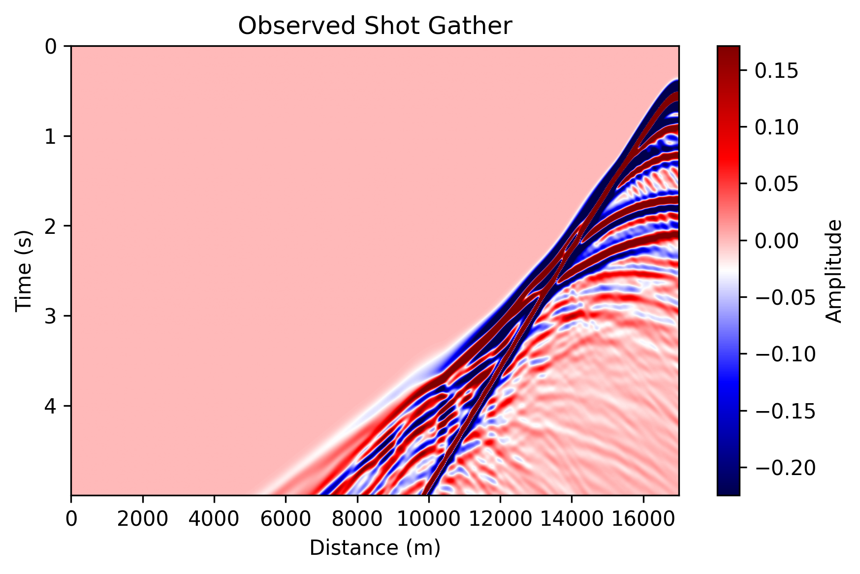
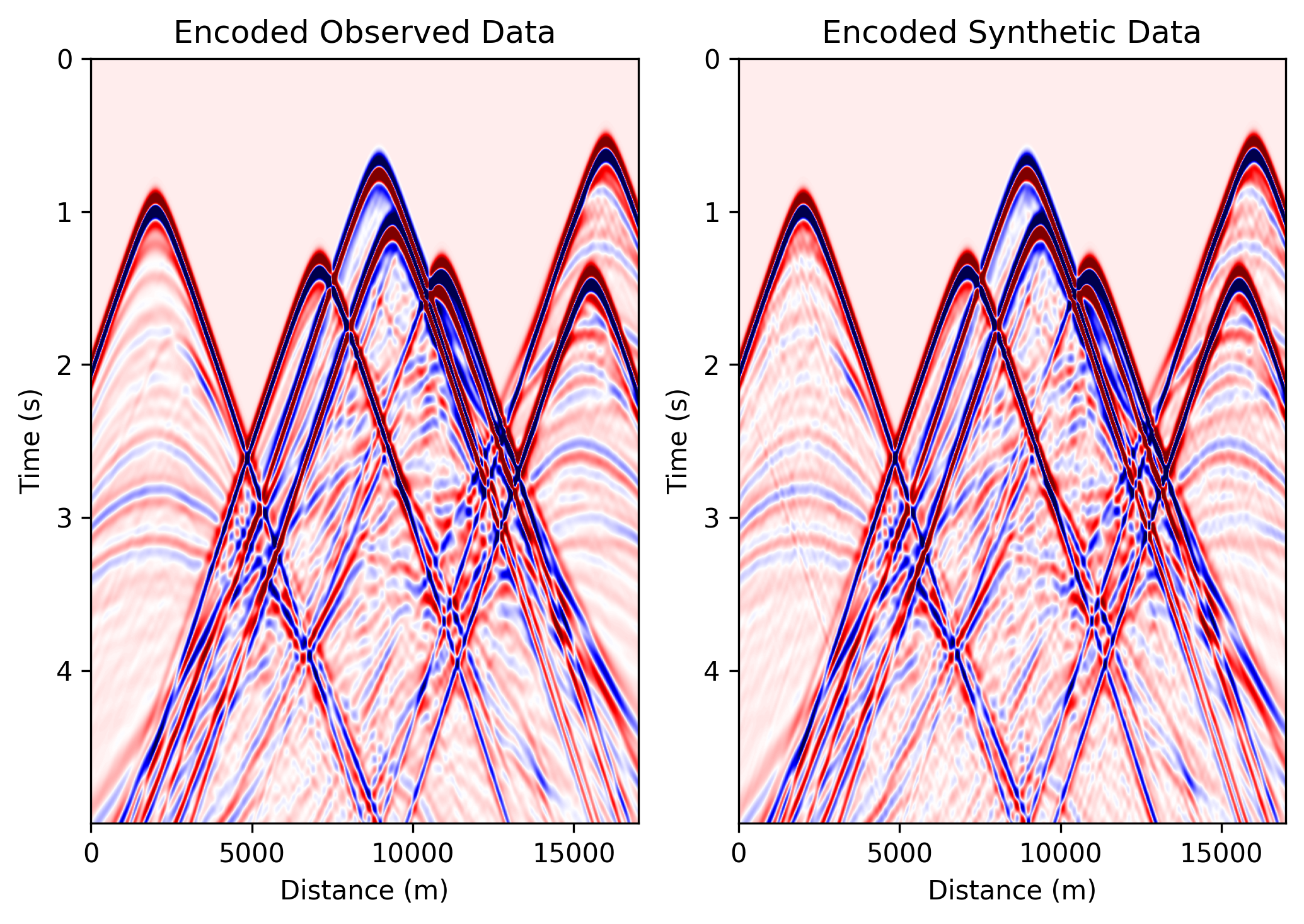
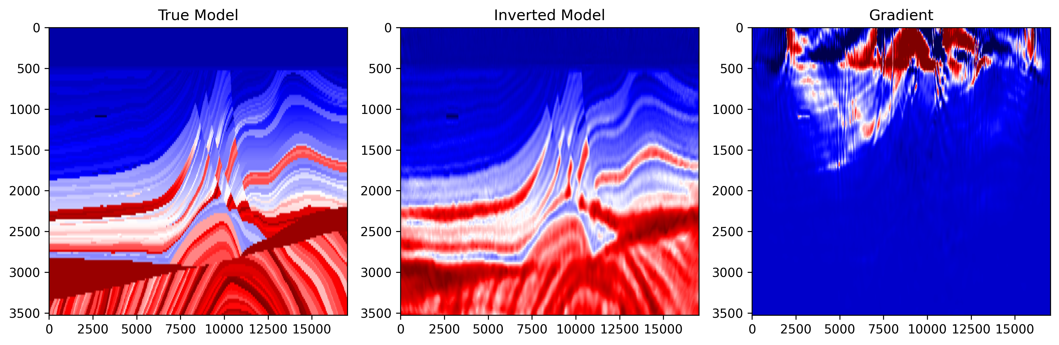
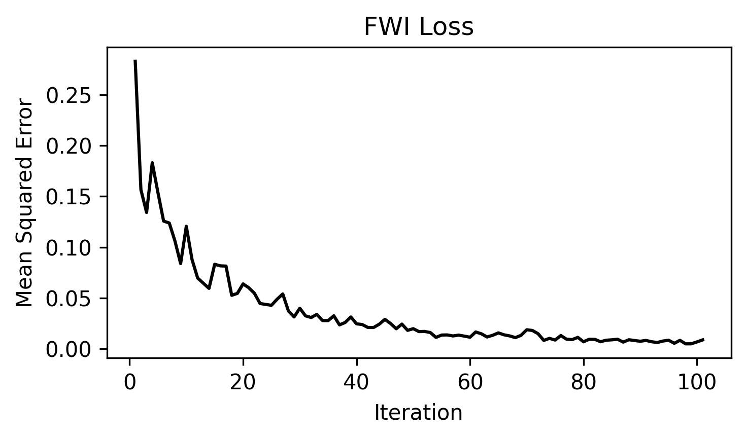
• ricker.png: Shows the Ricker wavelet used as the seismic source.
• observed_data.png: Shows one observed shot gather generated from the true velocity model.
• data_epoch_XXXX.png: Shows the encoded observed data and encoded synthetic data at a given epoch. This is useful for checking whether the synthetic data are gradually matching the encoded observations.
• epoch_XXXX.png: Shows three panels: 1) true model; 2) current inverted model; 3) current gradient. This figure helps monitor the inversion process.
• loss.png: Shows the FWI loss curve during optimization.

Example Figures

The following figures show one completed CUDA run from examples/reducingmemory/source_encoding/torch/acoustic_fwi_encoding_cuda/. The eager backend produces the same file set with the same naming pattern.

observed_data.png: one observed shot gather generated from the true Marmousi model.

data_epoch_0100.png: the encoded observed data and encoded synthetic data at a late inversion epoch, useful for checking whether the encoded prediction is matching the encoded target.

epoch_0100.png: the true model, inverted model, and gradient near the end of the run.

loss.png: the source-encoding FWI loss curve across optimization steps.

Main Configuration

Most parameters now come from the shared Marmousi configuration in examples/_shared/configure_marmousi.py. This example adds the source-encoding-specific output directories and max_time_shift_ratio there as well.

shared_config.get_config("fwi_2d_acoustic_encoding_torch_eager")
shared_config.get_config("fwi_2d_acoustic_encoding_torch_cuda")

Important parameters:

• nt, dt: These define the number of time samples and the time interval.
• fm, delay: These define the dominant frequency and delay of the Ricker wavelet.
• dh: This is the grid spacing of the velocity model.
• src_step, rec_step, srcz, recz: Acquisition geometry settings. src_step is source spacing in grid points; rec_step is the receiver spacing in grid points; srcz is source depth index; recz is receiver depth index.
• epochs, batchsize, lr: These control the number of inversion iterations, the number of shots used per encoded batch, and the learning rate.
• max_time_shift_ratio: This controls the maximum random time shift used in source encoding. For example, if nt=2500, then the maximum shift is: 0.2 × 2500 = 500.

Backend-Specific Settings

Backend-specific settings are defined in examples/_shared/configure_marmousi.py.

PyTorchCUDA

{
    "output_dir": "acoustic_fwi_encoding_eager",
    "use_ckpt": False,
    "use_compile": True,
    "transpose_shot": False,
}

This backend is useful for testing and debugging.

{
    "output_dir": "acoustic_fwi_encoding_cuda",
    "transpose_shot": True,
    "boundary_saving_config": {
        "enabled": True,
        "storage": "gpu",
        "transfer_interval": 10,
        "pinned_memory": True,
    }
}

The CUDA backend is intended for faster propagation.

Boundary saving is enabled to reduce memory usage during backpropagation.

Source Encoding Call Shapes

The eager and CUDA paths both support source encoding, but they expect different input layouts when source_encoding=True.

For the broader runtime shape conventions used by PropTorch, PropJax, and PropCUDA, see API Reference > Propagators.

EagerCUDA

The eager path keeps one encoded source per selected shot and collapses the selected shots internally.

Use:

• wavelet: (nsel, nt)
• sources: (nsel, 2)
• receivers: (1, nreceivers, 2)

Here nsel is the number of randomly selected shots in the current inversion step.

The CUDA path expects a single batch that already contains multiple encoded sources inside that batch.

Use:

• wavelet: (1, nsrc, nt)
• sources: (1, nsrc, 2)
• receivers: (1, nreceivers, 2)

Here nsrc is the number of encoded sources combined into the current super-shot.

In practice, the main difference is that eager passes selected sources as a plain shot list, while CUDA passes them as one batched encoded-source block.