2D Acoustic FWI on Marmousi with Torch

Source file:

• examples/FWI/2d/acoustic/torch/fwi_marmousi.py

What This Example Does

This example runs acoustic full-waveform inversion with one script that supports two propagator backends:

• eager: pure PyTorch propagation through PropTorch(..., backend="eager")
• cuda: compiled CUDA propagation through PropTorch(..., backend="cuda")

The script:

1. loads a true velocity model and a smooth initial model
2. builds an acoustic solver for the selected backend
3. generates observed data from the true model
4. inverts the initial model by matching synthetic and observed gathers

Main Components

The solver is built from:

• equation: Acoustic(...)
• propagator: PropTorch(...)
• wave: a Ricker wavelet
• sources: regularly sampled source coordinates
• receivers: regularly sampled receiver coordinates
• models: the velocity model vp

Prepare the Marmousi Model Files

This example reads:

• examples/models/marmousi/true.npy
• examples/models/marmousi/smooth.npy

Generate them from the official Elastic Marmousi archive before running the example:

python3 examples/models/marmousi/download_marmousi.py --extract
python3 examples/models/marmousi/extract_model_segy.py
python3 examples/models/marmousi/convert_segy_to_npy.py
python3 examples/models/marmousi/prepare_fwi_models.py \
  --input examples/models/marmousi/npy/vp_1p25m.npy \
  --source-dh 1.25 \
  --target-dh 25.0 \
  --radii 8,8 \
  --passes 3

Optional preview:

python3 examples/models/marmousi/plot_models.py

The generated model files under examples/models/ are ignored by git. The helper scripts in that directory remain tracked.

Backend Selection

Run the example with:

PyTorchCUDA

python3 examples/FWI/2d/acoustic/torch/fwi_marmousi.py --backend eager

python3 examples/FWI/2d/acoustic/torch/fwi_marmousi.py --backend cuda

The script keeps:

• COMMON_CONFIG: shared acquisition and inversion settings
• BACKEND_CONFIG: backend-specific options for the eager and CUDA paths

For BACKEND_CONFIG, the script uses:

• EagerOptions(...) for the eager path
• CUDAOptions(memory=...) for the CUDA path

Key Configuration

Shared configuration includes:

• nt, dt: temporal sampling
• dh: spatial sampling
• spatial_order: finite-difference order
• src_step, rec_step: acquisition sampling in the x direction
• true_model, init_model: .npy files loaded from examples/models/
• epochs, batchsize, lr: inversion hyperparameters

Backend-specific configuration includes:

• eager: EagerOptions(use_compile=...) and use_ckpt
• CUDA: CUDAOptions(memory=MemoryOptions(...)) and display transpose rules for saved figures

Solver Setup

The equation side is shared across both modes:

equation = Acoustic(
    spatial_order=cfg["spatial_order"],
    device=dev,
    backend="torch",
)

Even when the solver runs with backend="cuda", the equation backend remains "torch".

Shared propagator arguments are collected first:

prop_kwargs = dict(
    shape=shape,
    dev=dev,
    dh=cfg["dh"],
    dt=cfg["dt"],
    source_type=["h1"],
    receiver_type=["h1"],
    abcn=cfg["abcn"],
    free_surface=cfg["free_surface"],
    pml_type="cpmlr",
)

PyTorchCUDA

solver = PropTorch(
    equation,
    **prop_kwargs,
    use_ckpt=cfg["use_ckpt"],
    backend="eager",
    eager_options=EagerOptions(use_compile=cfg["use_compile"]),
)

solver = PropTorch(
    equation,
    **prop_kwargs,
    backend="cuda",
    cuda_options=CUDAOptions(
        memory=MemoryOptions(
            strategy="boundary",
            boundary=BoundaryOptions(...),
        )
    ),
)

Geometry

The example uses a fixed-depth surface acquisition:

• sources are placed every src_step grid points
• receivers are placed every rec_step grid points
• all sources use the same source depth srcz
• all receivers use the same receiver depth recz

The final array shapes are:

• sources: (nshots, 2)
• receivers: (nshots, nreceivers, 2)

Inversion Workflow

Observed data is generated first from the true model, then the inversion updates the smooth model with torch.optim.Adam.

At each iteration, the script:

1. selects a random subset of shots
2. computes synthetic data
3. evaluates the L2 data-misfit loss
4. backpropagates gradients to vp
5. updates the model

Outputs

The script creates an output directory under examples/ and saves:

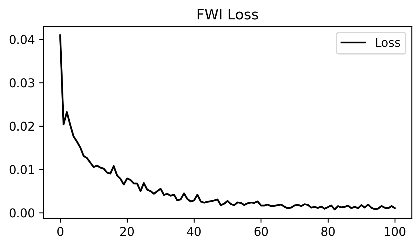
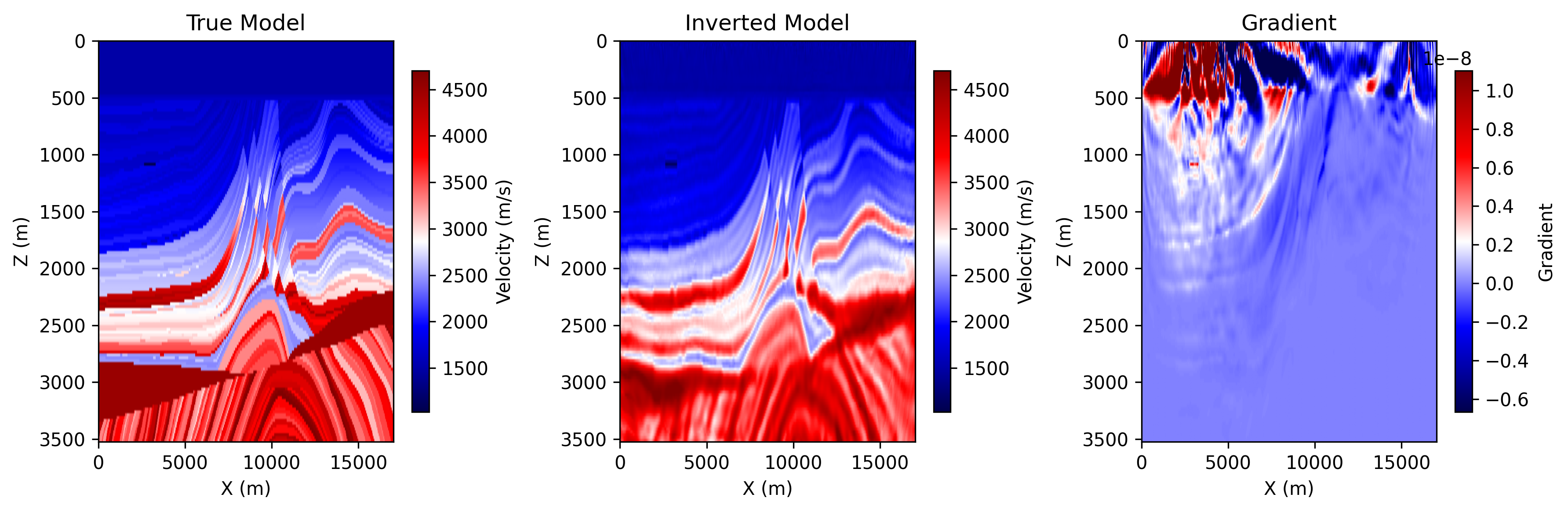
• ricker.png
• observed_data.png
• loss.png
• epoch_XXXX.png: includes the true model, the current inverted model, and the current gradient

Each backend writes into its own output directory:

PyTorchCUDA

acoustic_fwi_torch

acoustic_fwi_cuda

Example Figures

The following figures show two common outputs from a completed acoustic FWI run.

loss.png: the inversion loss curve across optimization steps.

epoch_0100.png: the saved progress panel at the final shown epoch, including the true model, the current inverted model, and the current gradient.

Running the Example

Step 1. Prepare the Marmousi .npy files listed above if they do not already exist.

Step 2. Choose the backend you want to use.

PyTorchCUDA

python3 examples/FWI/2d/acoustic/torch/fwi_marmousi.py --backend eager

python3 examples/FWI/2d/acoustic/torch/fwi_marmousi.py --backend cuda

Step 3. Check the output directory for the saved figures.

Notes:

• eager mode runs on GPU if available and otherwise falls back to CPU
• cuda mode requires a CUDA-capable PyTorch environment and compiled binding