GETTING STARTED
Your first FWI in five steps.
From a fresh terminal to running gradient descent on a toy velocity model. By the end you'll be ready to open any of the notebooks.
01
Install
Pick whichever backend you already have. SWEEP supports lazy imports — you don't need both PyTorch and JAX.
PyTorch backend
recommended
$ pip install "sweep[torch] @ git+https://github.com/DeepWave-KAUST/sweep.git"
JAX backend
$ pip install "sweep[jax] @ git+https://github.com/DeepWave-KAUST/sweep.git"
tip Not on PyPI yet — install straight from GitHub. For the compiled CUDA backend (
impl="c") or a dev clone, see
Install from source.
02
Build a velocity model
A simple 2-layer model: 1500 m/s in the top half, 2000 m/s below. 10 m grid spacing.
quickstart.py
import torch, numpy as np
from sweep.propagator.torch import PropTorch
from sweep.equations       import Acoustic
from sweep.signal          import ricker

# A 2-layer 100×100 model.
vp = np.ones((100, 100), dtype=np.float32) * 1500
vp[50:, :] = 2000

vp · 100 × 100 · 10 m grid
03
Run a forward shot
Construct the equation, wrap it in a propagator, and call forward().
propagator
eq   = Acoustic(spatial_order=8, device="cuda", backend="torch")
prop = PropTorch(eq, shape=(100, 100), dev="cuda", dh=10., dt=2e-3,
                 source_type=["h1"], receiver_type=["h1"], pml_type="cpmlr")

wave      = ricker(np.arange(0, 1.5, 2e-3) - 0.1, f=8)
sources   = np.array([[50, 2]])
receivers = np.array([[[ix, 2] for ix in range(10, 90)]])

obs = prop.forward(wave, sources, receivers, models=[torch.from_numpy(vp).to("cuda")])
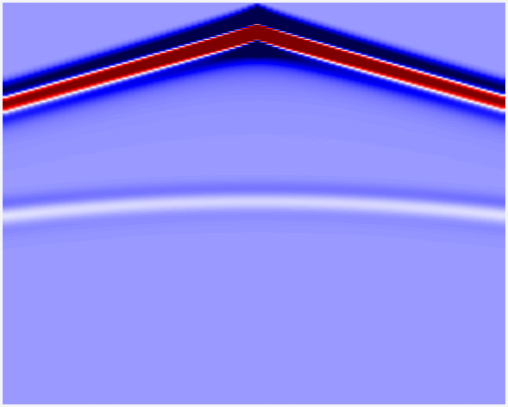
shot record · 1 src · 1 rec · 750 samples
04
Get the gradient
Tag vp with requires_grad_, run forward, and backward(). That's it.
vp_t = torch.from_numpy(vp).to("cuda").requires_grad_(True)
obs  = prop.forward(wave, sources, receivers, models=[vp_t])
obs.pow(2).sum().backward()

# vp_t.grad now holds the sensitivity kernel.
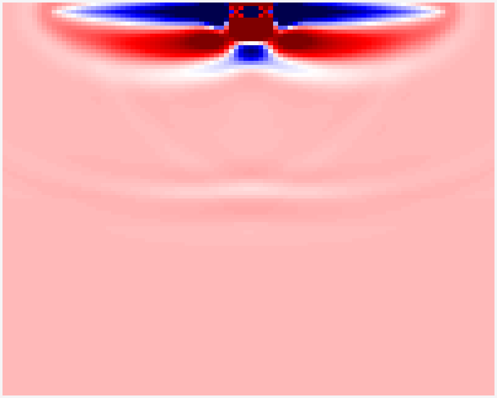
∂L/∂vp · 100 × 100
05